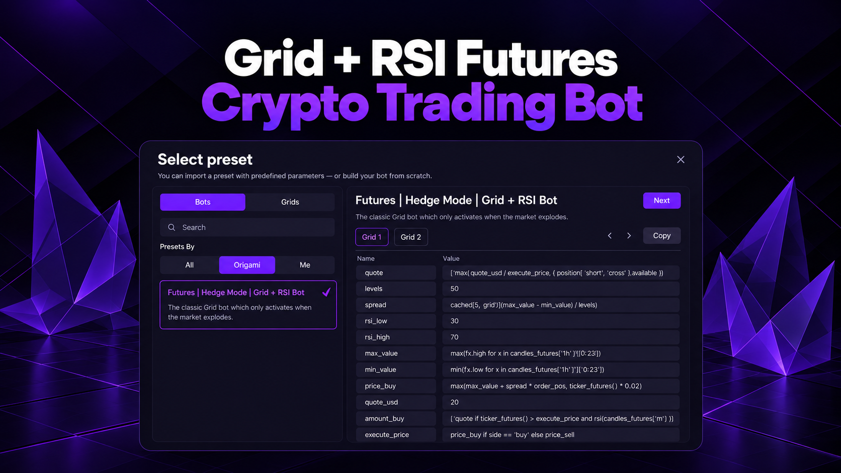
The Futures | Hedge Mode | Grid + RSI Bot is an Origami Tech crypto trading bot preset that combines dynamic grid execution, RSI conditions and independent long and short position management.

The preset contains two separate grids. One manages the long side and the other manages the short side. Each grid can track its own position, notional exposure, break even price, entry levels and exit conditions.

The default configuration uses 50 grid levels, RSI thresholds of 30 and 70, a USD based quote value of 20, and a dynamic price range calculated from recent hourly futures candles. Origami Tech describes the preset as a strategy for strong directional moves and breakouts from recent price ranges.

This guide explains how the crypto trading bot calculates its grid, how the visible Grid 1 formulas work, which parameters can be adjusted and what to monitor after launch.

What Is the Grid + RSI Futures Crypto Trading Bot?

The strategy combines three types of information.

First, it analyzes recent futures prices to calculate a working market range.

Second, it divides that range into multiple grid levels.

Third, it combines those levels with RSI and current position data to determine order prices and volumes.

The preset operates in Hedge Mode, so long and short positions can be managed independently. Origami Tech confirms that the strategy uses two separate 50 level grids and separate position logic for the two sides.

The preset contains two mirrored grids. Grid 1 manages the long position, while Grid 2 manages the short position. Both use the same 50 level structure, RSI thresholds and dynamic market range, while maintaining separate position and exit calculations.

‍

Its core variables include:

levels = 50
rsi_low = 30
rsi_high = 70
quote_usd = 20

The rest of the values are calculated dynamically from price history and the current position.

How Grid 1 Calculates the Market Range

The grid begins by reading recent hourly futures candles.

The visible upper boundary formula is:

max_value =
max([x.high for x in candles_futures('h1')][0:23])

The bot therefore looks at the highs of the recent hourly candles and takes the maximum value.

The lower boundary follows the same general structure using candle lows. The interface cuts off the right side of the full formula, so only the visible portion can be quoted exactly:

min_value =
min([x.low for x in candles_futures('h1')][0:23]) ...

The important point is that the grid range is based on recent hourly market data.

This gives the crypto trading bot a dynamic upper and lower boundary instead of relying on permanent fixed price levels.

Origami Tech also describes the preset's market range as dynamically calculated from recent hourly futures candles.

Why the Hourly Range Matters

Suppose the recent candle data produces:

max_value = 110
min_value = 100

The total range is:

110 - 100 = 10

That range becomes the basis for calculating the distance between grid levels.

If volatility expands and the observed range becomes larger, grid spacing also grows.

If the recent market range contracts, the grid becomes tighter.

Number of Grid Levels

The default is:

levels = 50

Grid 1 therefore prepares 50 buy levels.

The visible formula later confirms this directly:

buy_orders_count = levels

With the default configuration:

buy_orders_count = 50

This is an important difference from presets that work with only one active entry order.

The Grid + RSI crypto trading bot can calculate many potential entry levels across its current dynamic range.

Dynamic Grid Spread

The preset calculates the distance between levels with:

spread =
cached(5, 'grid')((max_value - min_value) / levels)

At its core, the calculation is:

(max_value - min_value) / levels

Using the previous example:

max_value = 110
min_value = 100
levels = 50

the grid distance would be:

(110 - 100) / 50 = 0.2

Each consecutive level can therefore be separated by approximately 0.2 price units before other strategy conditions are applied.

The cached(5, 'grid') part indicates that Origami Tech caches the calculation inside the grid logic rather than recalculating every component continuously.

RSI Thresholds

The preset uses:

rsi_low = 30
rsi_high = 70

These are standard lower and upper RSI reference levels.

The complete amount_buy formula visible in the interface is cut off, although its visible section clearly includes an RSI condition:

amount_buy =
(quote if ticker_futures() > execute_price
and rsi(candles_futures(...))
...

This confirms that order sizing or activation depends on both current price conditions and RSI logic.

Origami Tech's public preset page also confirms that RSI 30 and RSI 70 are included in both grid strategies together with price and position conditions. origami.tech

What Happens When You Change RSI?

A lower rsi_low, for example:

rsi_low = 25

makes the lower RSI condition more selective.

A higher value such as:

rsi_low = 35

allows the relevant long logic to react under less extreme RSI conditions.

The same principle applies to rsi_high.

Increasing:

rsi_high = 75

requires a stronger upper RSI reading.

Reducing it:

rsi_high = 65

makes the upper condition easier to reach.

Because the preset combines RSI with grid and position conditions, changing these values modifies signal frequency rather than simply shifting a single entry price.

Buy Price Formula

The visible Grid 1 formula is:

price_buy =
max(
   max_value + spread * order_pos,
   ticker_futures() * 0.02
)

This formula uses three important inputs:

max_value
spread
order_pos

Each grid order receives a position inside the grid through order_pos.

The calculation:

max_value + spread * order_pos

creates a different price for each order position.

With 50 order levels, each order can therefore receive its own dynamically calculated execution level.

The formula also compares that value with:

ticker_futures() * 0.02

and selects the higher result through max().

This behavior is part of the current preset formula and should be preserved when describing the original strategy.

USD Based Order Sizing

The default value is:

quote_usd = 20

The visible quote calculation begins as:

quote =
max(
   quote_usd / execute_price,
   position('short', 'cross').available
)

The formula connects the USD based quote amount with the execution price and existing opposite side position data.

The first part:

quote_usd / execute_price

converts the USD based order value into base asset quantity.

For example, if:

quote_usd = 20
execute_price = 2000

then:

20 / 2000 = 0.01

The basic quantity associated with a 20 USD quote value would therefore be 0.01 units.

The max() function also compares this value with available short position data.

This is one example of how Hedge Mode position state is incorporated directly into the grid calculations.

Long Position Data

Grid 1 explicitly defines:

position_long =
position(
   position_side='long',
   margin_mode='cross'
)

The strategy therefore reads a long futures position using cross margin.

From that object, the crypto trading bot obtains information such as:

position_long.available_quantity
position_long.breakeven_price
position_long.notional_usd

These values affect both position management and exit calculations.

Long Notional

The visible formula is:

long_notional =
cached(5, 'grid')(position_long.notional_usd)

This stores the current USD notional value of the long position.

Position notional is useful for monitoring how much exposure has accumulated as different grid levels execute.

Long Break Even Price

The preset also calculates:

long_bep =
cached(5, 'grid')(position_long.breakeven_price)

This represents the break even price of the entire long position.

Once several grid orders have filled at different prices, the relevant reference becomes the combined position break even price rather than the price of one individual order.

Dynamic Take Profit

One of the most useful formulas in the preset is:

take_profit =
spread / position_long.breakeven_price

This means the take profit distance is connected directly to current grid spacing.

The bot does not use one permanently fixed percentage.

Instead, take_profit changes as:

spread

and:

position_long.breakeven_price

change.

For example:

spread = 2
position_long.breakeven_price = 2000

produces:

2 / 2000 = 0.001

or:

0.1%

If grid spacing widens, the corresponding take profit distance can also become larger.

This keeps the exit logic connected to the structure of the active grid.

Sell Price and Long Exit

Grid 1 uses:

price_sell =
max(
   position_long.breakeven_price * (1 + take_profit),
   ticker_futures()
)

This formula calculates a sell target using the long position break even price plus the dynamically calculated take profit.

The first part is:

position_long.breakeven_price * (1 + take_profit)

Suppose:

break even = 2000
take_profit = 0.001

The calculated profit price becomes:

2000 * 1.001 = 2002

The formula then compares that value with the current futures ticker and uses the higher price.

This creates a dynamic exit target for the long position.

Sell Amount

The exit amount is straightforward:

amount_sell =
position_long.available_quantity

The strategy therefore uses the available long quantity as its sell amount.

This allows the exit side to reference the actual current position instead of a fixed USD amount.

When the Exit Order Is Active

The visible formula is:

sell_orders_count =
1 if position_long.available_quantity > 0 else 0

The bot creates one sell order when a long position exists.

When:

position_long.available_quantity = 0

the sell order count becomes zero.

When:

position_long.available_quantity > 0

one exit order becomes active.

This creates a clear distinction between the entry grid and the exit logic.

The strategy can have:

50 buy grid orders

and:

1 long exit order

once long exposure exists.

Final Execution Price

The preset uses:

execute_price =
price_buy if side == 'buy' else price_sell

For entry grid orders:

execute_price = price_buy

For the exit:

execute_price = price_sell

The same grid can therefore calculate both entry and exit execution through one final price variable.

Final Execution Volume

The formula is:

execute_volume =
amount_buy if side == 'buy' else amount_sell

For a buy order:

execute_volume = amount_buy

For a sell order:

execute_volume = position_long.available_quantity

This allows entry volume and exit volume to follow different sizing rules.

Grid 1 Default Parameters

What Does One Grid Cycle Look Like?

Assume the recent hourly futures range is:

min_value = 1900
max_value = 2000

with:

levels = 50

The basic grid spacing becomes:

(2000 - 1900) / 50 = 2

Now suppose several grid orders fill and the combined long position has:

position_long.breakeven_price = 1950

The dynamic take profit becomes:

2 / 1950 ≈ 0.001026

or approximately:

0.103%

The basic profit reference becomes:

1950 * (1 + 0.001026)
≈ 1952

The sell price formula then compares that value with the current futures ticker.

The bot can therefore maintain multiple dynamically spaced entry orders while managing the accumulated long position through one break even based exit.

How Grid 2 Manages the Short Position

Grid 2 mirrors the overall architecture of Grid 1 but manages the short side of the Hedge Mode strategy.

While Grid 1 creates multiple buy levels and manages the resulting long position, Grid 2 creates multiple sell levels and manages the resulting short position.

The default parameters remain:

levels = 50
rsi_low = 30
rsi_high = 70
quote_usd = 20

Grid 2 also uses the same dynamic market range based on recent hourly futures candles.

Dynamic Market Range

The lower boundary is calculated from recent hourly candle lows:

min_value =
min([x.low for x in candles_futures('h1')][0:23])

The upper boundary is also based on the highs of the recent hourly futures candles.

The exact right side of the max_value expression is partially hidden in the preset interface, while the visible logic confirms that the same recent hourly market range is used by Grid 2.

The distance between grid levels is calculated as:

spread =
cached(5, 'grid')((max_value - min_value) / levels)

With:

levels = 50

the current market range is divided into 50 price intervals.

This gives Grid 2 a dynamic sell grid that expands or contracts as the recent futures range changes.

Short Entry Grid

The sell grid uses:

price_sell =
min_value + spread * order_pos

Each order receives its own order_pos, so the formula creates a different sell price for every level.

With 50 levels:

sell_orders_count = levels

which means Grid 2 can generate up to 50 sell levels.

Suppose:

min_value = 100
spread = 2

An order at:

order_pos = 3

would use:

100 + 2 * 3 = 106

as its calculated grid price before the other strategy conditions are applied.

This is the short side equivalent of the long entry grid in Grid 1.

RSI Conditions for the Short Grid

Grid 2 uses the same RSI thresholds:

rsi_low = 30
rsi_high = 70

The visible amount_sell formula also contains both a futures price comparison and an RSI condition.

Its full expression extends beyond the visible width of the preset interface, so the exact code should not be reconstructed from the screenshot.

The confirmed behavior is that sell order sizing depends on the current grid price together with RSI based conditions.

This allows the crypto trading bot to combine dynamic grid levels with indicator based execution rather than treating every calculated sell level as automatically executable.

Short Position

Grid 2 reads the short futures position directly:

position_short =
position(
   position_side='short',
   margin_mode='cross'
)

This position object provides the strategy with information about the current short exposure.

Important values include:

position_short.available_quantity
position_short.breakeven_price
position_short.notional_usd

These values are used to manage both the existing short position and its exit.

Short Notional

The preset tracks:

short_notional =
position_short.notional_usd

This represents the USD notional value of the current short position.

As additional sell levels execute, the total short exposure can increase.

Monitoring short_notional therefore helps show how much exposure has accumulated across the Grid 2 entry levels.

Short Break Even Price

The preset defines:

short_bep =
position_short.breakeven_price

This is the break even price of the combined short position.

After several sell orders execute at different prices, the strategy can use the resulting break even price rather than the price of an individual entry.

This value becomes the reference point for the short exit calculation.

Dynamic Take Profit for the Short Position

Grid 2 calculates:

take_profit =
spread / position_short.breakeven_price

This mirrors the long side logic.

The profit distance therefore changes with both the current grid spacing and the short position break even price.

For example:

spread = 2
short break even price = 2000

gives:

2 / 2000 = 0.001

or:

0.1%

The wider the grid becomes, the larger the corresponding profit distance can become.

Short Exit Price

The buy price used to close the short position is:

price_buy =
min(
   position_short.breakeven_price * (1 - take_profit),
   ticker_futures()
)

For a short position, profit occurs when the asset price falls below the entry level.

The formula therefore calculates an exit below the short break even price.

Suppose:

short break even price = 2000
take_profit = 0.001

The calculated profit reference becomes:

2000 * (1 - 0.001) = 1998

The formula then compares that level with the current futures ticker and uses the lower value.

This creates a dynamic buyback price for closing the short position.

Short Exit Amount

The preset uses:

amount_buy =
position_short.available_quantity

The buy order used for the exit therefore matches the available short position quantity.

This allows the crypto trading bot to manage the current short exposure directly rather than using the fixed quote_usd value for the closing order.

When the Short Exit Becomes Active

The preset uses:

buy_orders_count =
1 if position_short.available_quantity > 0 else 0

When a short position exists, one buy order becomes active for the exit.

At the same time, the entry side uses:

sell_orders_count = levels

With the default settings, Grid 2 therefore combines:

50 potential sell grid orders

with:

1 short exit order

once short exposure exists.

Final Execution Price and Volume

Grid 2 uses the same directional selector structure as Grid 1:

execute_price =
price_buy if side == 'buy' else price_sell

For sell grid orders:

execute_price = price_sell

For the short exit:

execute_price = price_buy

Execution volume is selected through:

execute_volume =
amount_buy if side == 'buy' else amount_sell

This separates the sizing logic used for building a short position from the quantity used to close it.

How Grid 1 and Grid 2 Work Together

The two grids form a mirrored Hedge Mode structure.

Grid 1 manages the long side:

50 buy levels
1 sell exit
position_long
long_bep
long_notional

Grid 2 manages the short side:

50 sell levels
1 buy exit
position_short
short_bep
short_notional

Both grids share the same core settings:

levels = 50
rsi_low = 30
rsi_high = 70
quote_usd = 20

Both also use the recent hourly futures range to calculate:

max_value
min_value
spread

The major difference is direction.

Grid 1 builds long exposure through buy levels and exits through a sell order above the long break even price.

Grid 2 builds short exposure through sell levels and exits through a buy order below the short break even price.

This is what allows the crypto trading bot to maintain and manage long and short futures positions independently in Hedge Mode.

Grid 2 Default Logic

Which Markets Are Suitable for This Crypto Trading Bot?

The Grid + RSI preset is designed for futures markets where dynamic grids and Hedge Mode are supported.

Origami Tech positions the strategy around:

• strong directional moves
• breakouts from recent price ranges
• liquid futures markets
• markets that can support multiple grid orders
• separate long and short position management

Liquidity is especially important because one grid can contain 50 entry levels.

A strong movement can execute several grid orders and increase total position exposure.

Markets with sufficient order book depth generally provide a more stable environment for this type of crypto bot trading strategy.

Which Parameters Should You Change?

levels

Default:

50

Increase this parameter when you want more grid levels within the same market range.

More levels reduce the average distance between orders.

For example:

levels = 100

would halve the basic spread compared with 50 levels if max_value and min_value remain unchanged.

Reducing the number of levels makes the grid less dense.

This can reduce the number of potential fills during one market move.

quote_usd

Default:

20

This is the clearest sizing input in the preset.

Increasing it raises the USD based quantity used by entry calculations.

Reducing it lowers the size of individual grid executions.

For accounts with smaller risk limits, reducing quote_usd can slow the growth of total position exposure.

rsi_low

Default:

30

A lower value creates a more selective lower RSI condition.

A higher value makes the condition easier to reach.

rsi_high

Default:

70

A higher value creates a more selective upper RSI condition.

A lower value increases the number of market situations that can satisfy it.

levels and quote_usd Together

These two parameters deserve to be evaluated together.

For example:

50 levels × 20 USD

creates a very different maximum potential order structure from:

100 levels × 50 USD

Increasing both parameters simultaneously can materially increase potential futures exposure.

The number of levels should therefore always be considered together with individual order sizing.

Parameters That Change the Strategy More Deeply

Values such as:

max_value
min_value
spread
price_buy
price_sell
take_profit
execute_price

form the structural logic of the crypto trading bot.

Changing the hourly candle range affects the market structure used by the grid.

Changing spread modifies the relationship between all grid levels.

Changing take_profit modifies how exits are derived from the accumulated position.

Changing price_buy or price_sell changes the actual execution model.

These adjustments are better treated as modifications to the underlying crypto bot trading strategy rather than routine preset tuning.

How to Launch the Grid + RSI Crypto Trading Bot

Create or open an Origami Tech project.

Connect an exchange account that supports futures crypto trading and Hedge Mode.

Create a futures crypto trading bot and configure:

• exchange account
• futures pair
• Hedge Mode
• margin mode
• leverage

Open the preset library and choose:

Futures | Hedge Mode | Grid + RSI Bot

Review both Grid 1 and Grid 2.

Pay particular attention to:

levels
quote_usd
rsi_low
rsi_high
spread
long_notional
short_notional
long_bep
short_bep
take_profit

Then review the resulting orders and total potential exposure before enabling the crypto trading bot.

What to Monitor After Launch

The key values to follow are:

• active grid orders
• long position size
• short position size
• long_notional
• short_notional
• long_bep
• short_bep
• realized PnL
• unrealized PnL
• current RSI
• current dynamic range
• grid spread
• crypto trading fees
• funding costs

Origami Tech provides position, order, realized PnL and unrealized PnL monitoring for active strategies.

Main Risks

A 50 level grid can accumulate several fills during a rapid market movement.

Each fill changes total exposure and the break even price of the position.

Hedge Mode can maintain long and short positions independently, which means total account exposure may include both sides simultaneously.

RSI conditions also remain market signals rather than guarantees of reversal.

Leverage, funding, liquidation risk and crypto trading fees should therefore be monitored together with grid parameters.

The most important risk variables are usually:

levels
quote_usd
leverage
total long notional
total short notional

Final Thoughts

The Futures | Hedge Mode | Grid + RSI Bot is a relatively sophisticated Origami Tech crypto trading bot preset because it combines a dynamically calculated futures range, 50 grid levels, RSI conditions and separate Hedge Mode position management.

The two grids show how these elements work together in Hedge Mode. Grid 1 builds long exposure through up to 50 buy levels and manages that position with one dynamic sell exit. Grid 2 mirrors the structure by building short exposure through up to 50 sell levels and managing that position with one dynamic buy exit.

Each side tracks its own position quantity, notional exposure and break even price. The dynamic take_profit calculation connects exit distance to current grid spacing on both sides:

long take_profit =
spread / position_long.breakeven_price

short take_profit =
spread / position_short.breakeven_price

This gives the crypto trading bot separate long and short execution systems while keeping both grids tied to the same recent futures market range, RSI thresholds and order sizing framework.

levels = 50
rsi_low = 30
rsi_high = 70
quote_usd = 20

For the long side, the crypto trading bot tracks position_long, long_notional and long_bep.

Its exit target is dynamic:

take_profit =
spread / position_long.breakeven_price

and:

price_sell =
max(
   position_long.breakeven_price * (1 + take_profit),
   ticker_futures()
)

This ties the exit logic directly to both grid spacing and the actual break even price of the accumulated position.

For routine configuration, levels, quote_usd, rsi_low and rsi_high are the clearest variables to review.

Changes to range calculations, grid spread, execution price formulas or dynamic exit logic represent deeper modifications to the underlying crypto trading bot strategy.

‍

General disclaimer: Futures crypto trading involves market, leverage, liquidation, funding, crypto trading fee and execution risks. Multiple grid fills can increase exposure quickly. Crypto trading bot presets automate predefined logic and do not guarantee profitability or future crypto trading bot returns.

‍